library(statnet)
data(florentine)Network communities
So far, we have only seen exogeneous groupings, such as office affiliation. We can instead also try to infer a grouping from the network which endogeneously identifies cohesive subgroups or communities.
In the following, we will walk through a couple of different approaches based on our network of florentine families.
The network contains an isolated node, which we remove because it will most usefully be classified to belong to its own singleton community:
noisol <- seq(network.size(flomarriage))[-isolates(flomarriage)]
flomarriage <- flomarriage %s% noisol
Hierarchical clustering
A very general approach towards identifying groups of similar objects is hierarchical clustering, which is also frequently used for applications outside of network analysis.
It involves two steps:
First, the specification of a distance matrix, which tells us for each pair of nodes how ‘close’ they are to each other. A simple measure to specify this would be the geodesic distance, which we can compute using the geodist function:
dist_gd <- geodist(flomarriage)$gdistKnowing the distance among all pairs of nodes and starting out with each node in its own cluster, we can now iteratively merge together the closest clusters of nodes, until all nodes are in the same cluster. To specify which clusters to merge, we need to define a so called linkage criterion. Two popular options are:
- average: merge clusters with the lowest average distance
- ward: merge clusters that result in the smallest total within-cluster variance
We can specify the linkage criterion by specifying the method argument to the hclust function, which will perform the clustering. We furthermore wrap our matrix of geodesic distances in the as.dist(...) function:
clust <- hclust(as.dist(dist_gd), method = "ward.D2")The iterative procedure described above will not only produce a single clustering of nodes, but instead gives us a hierarchy of groupings. We can inspect that hierarchy with a dendrogram to help us pick a sensible clustering:
plot(clust)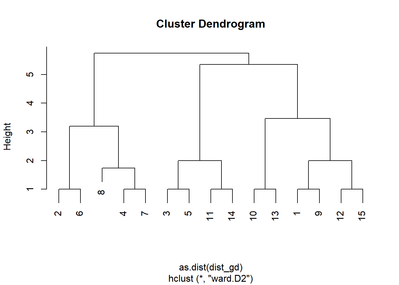
We can ‘cut’ this dendrogram at a specified hight h or indicate a given number of groups k to yield. Here, we go for three groups:
memb <- cutree(clust, k=3)Inspect result
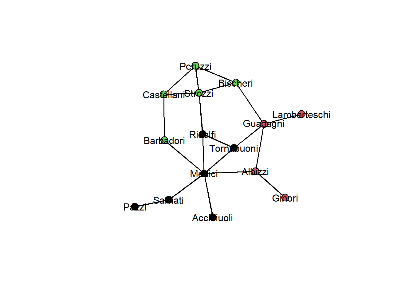
We can now inspect our detected communities by coloring nodes in the network graph:
gplot(flomarriage,
      gmode="graph",
      vertex.col=memb,
      displaylabels=TRUE, label.pos=5)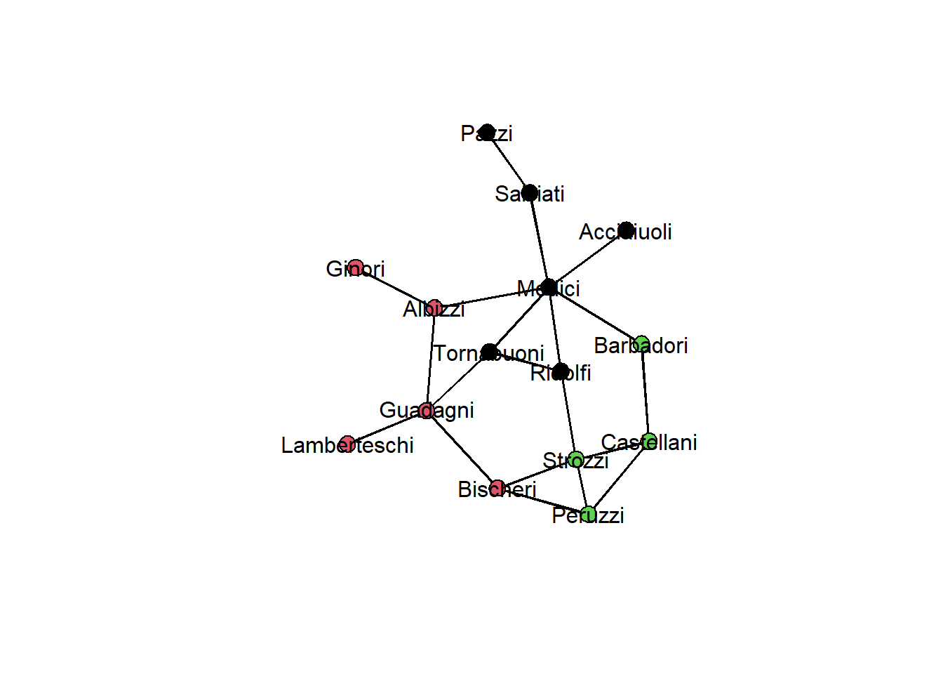
Alternatively, we could create a blockmodel by directly passing the cluster object and the desired number of groups:
bm <- blockmodel(flomarriage, clust, k=3)We can then plot the permuted adjacency matrix, as seen last session:
par(pty="s") # square plotting area for gridlines
plot(bm)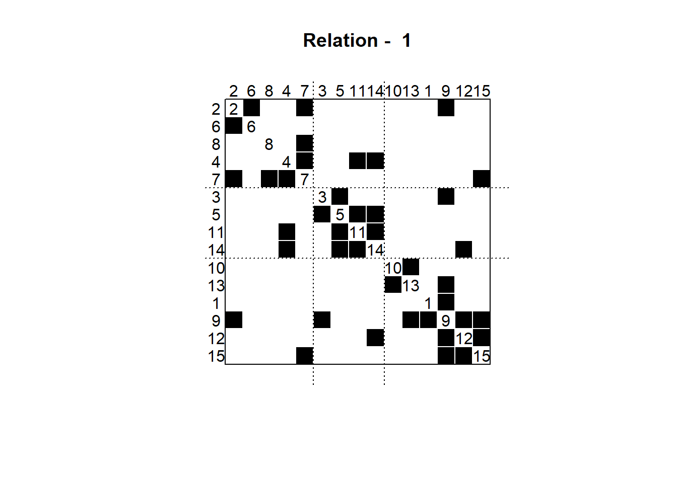
Modularity optimization
Specifying a distance matrix and using hierarchical clustering is a very flexible procedure, since we could easily plug in something other than geodetic distances to measure how ‘close’ to nodes are to each other (e.g., reachability, clique comembership, maximum flow). However, this approach does not scale beyond maybe a couple thousands of nodes and thus is not suitable for large networks.
Another popular approach is modularity optimization. Modularity measures the degree to which a network can be partitioned into internally cohesive and externally sparse subgroups. It does so by comparing the realized network structure to a random distribution of edges. This measure can then be taken as an optimization target to find a clustering for which the modularity is maximal, which is done, e.g., by the Louvain or the Leiden algorithm.
statnet does not implement modularity optimization, but igraph does. If we want to switch between the two, the intergraph package provides convenience methods for conversion:
library(intergraph)With this package, we can simply call asIgraph on a network object to produce a corresponding igraph graph object:
flomarriage_ig <- asIgraph(flomarriage)
flomarriage_ig
IGRAPH b9991a0 U--- 15 20 --
+ attr: na (v/l), priorates (v/n), totalties (v/n), vertex.names (v/c),
| wealth (v/n), na (e/l)
+ edges from b9991a0:
[1] 1-- 9 2-- 6 2-- 7 2-- 9 3-- 5 3-- 9 4-- 7 4--11 4--14 5--11
[11] 5--14 7-- 8 7--15 9--12 9--13 9--15 10--13 11--14 12--14 12--15We can then call igraph functions on this object, such as the cluster_louvain(...) method for modularity optimization:
clust_ig <- igraph::cluster_louvain(flomarriage_ig) From this clustering object we can then extract the membership vector:
membership_louvain <- igraph::membership(clust_ig)As before, we can investigate the result, e.g., by using node colors:
gplot(flomarriage,
      gmode="graph",
      vertex.col=membership_louvain,
      displaylabels=TRUE, label.pos=5)