library(network)
library(sna)
library(readr)Different Types of Networks
Networks can be categorized in various ways depending on their characteristics. We will cover three types of networks here: directed and undirected networks, weighted and unweighted networks, and unipartite and bipartite networks.
As usual, we start by loading the necessary packages into our session:
Directed and undirected networks
A directed network (or digraph) is a network where the edges have a direction, i.e., they distinguish between a source and a target node. Inherent asymmetry of ties is the case for many real world networks, such as advice giving, money lending, or the transmission of infectious diseases.
However, not all relations are inherently asymmetric (e.g., friendships), and sometimes it is necessary to drop edge directions for analytic reasons.
In R, we can specify upon construction whether a network should be directed or not, using the directed = TRUE/FALSE flag. E.g. for this data frame representing an edgelist:
edgelist <- data.frame(
  sender   = c(1,1,2,2,3,3,3),
  receiver = c(2,3,1,4,1,2,4)
)
We can construct a directed network in the following way:
directed <- network(edgelist, directed = TRUE)Symmetrization
If we have a directed network but want an undirected one, we can symmetrize it. Networks can be symmetrized in multiple different ways, with the two common rules being the “weak” rule and the “strong” rule.
Weak rule symmetrization is the more permissive approach and adds an undirected edge between two nodes if there is an edge in at least one direction in the original network. In contrast, the strong rule requires an edge to be present in both directions for the edge to be present in the symmetrized network.
Symmetrization can be achieved in R using the symmetrize(...) function:
adj_sym <- symmetrize(directed, rule = "weak")Since this function returns a symmetrized adjacency matrix, we also need to reconstruct our network if we want a network object, where we also explicitly pass directed = FALSE:
net_sym <- network(adj_sym, directed=FALSE)Plotting directed and undirected networks
Directed edges are usually represented by arrows in a network plot. If we pass a directed network to gplot(...), this is the default (because the default value of the gmode argument is digraph):
gplot(directed, label = 1:4)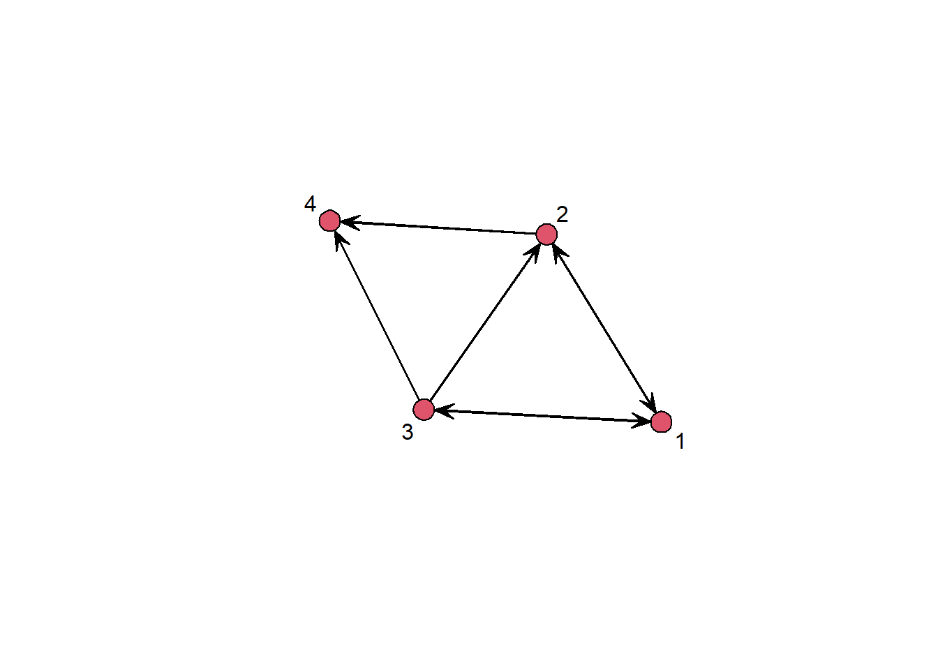
If we want to plot an undirected network, we include gmode = "digraph" in the call to gplot:
gplot(net_sym, gmode = "graph", label = 1:4)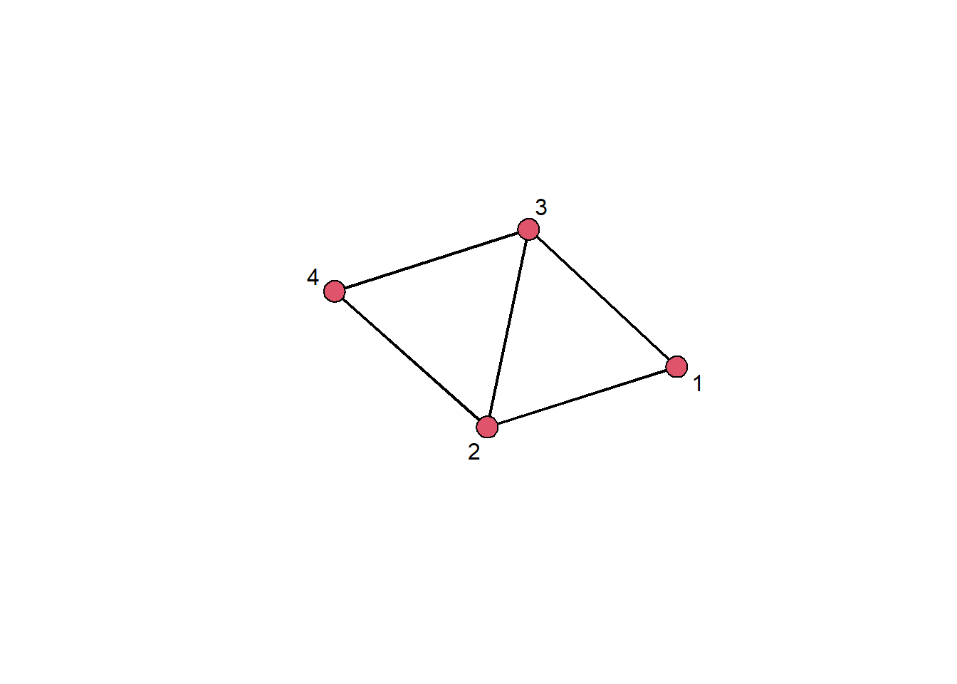
Weighted and unweighted networks
A weighted network is a network where the edges have weights representing the strength or intensity of the relationship between nodes.
Similarly to directed networks, edge weights are common in many real-world scenarios, such as transportation or trade networks, where weights could represent the distance or trade volume between countries.
The easiest way to construct a weighted network in R is by passing an adjacency matrix to the network function where the cells represent edge weights and not just the presence or absence of an edge.
To demonstrate, we can simulate a weighted adjacency matrix with random values:
adj_weighted <- matrix(rnorm(16), nrow = 4, ncol = 4)
adj_weighted
[,1] [,2] [,3] [,4]
[1,] 0.1713139 -1.7715350 1.2991695 0.7521626551
[2,] -0.1018933 0.0500760 1.6947802 0.3371616288
[3,] -0.3799781 0.7162077 -0.2425720 0.4156102367
[4,] 0.4359230 -0.6286307 -0.1554461 -0.0009468474By default, the network(...) function ignores edge values/weights. We here accordingly specify ignore.eval = FALSE and specify a name for our weights by setting names.eval = "name":
net_weighted <- network(adj_weighted,
                        ignore.eval = FALSE,
                        names.eval = "weight")
net_weighted
Network attributes:
vertices = 4
directed = TRUE
hyper = FALSE
loops = FALSE
multiple = FALSE
bipartite = FALSE
total edges= 12
missing edges= 0
non-missing edges= 12
Vertex attribute names:
vertex.names
Edge attribute names:
weight Dichotomization
If we have a weighted network but want a simple unweighted network, where edges are either present or not, we can dichotomize the adjacency matrix. This just means picking a threshold value and keeping all edges above that value while discarding the rest.
We can accomplish this in R using the ifelse(...) function, which checks a condition and returns one or another value depending on whether it is met:
thresh <- 0.3 # threshold value
adj_dicho <- ifelse(adj_weighted > thresh, 1, 0)
adj_dicho
[,1] [,2] [,3] [,4]
[1,] 0 0 1 1
[2,] 0 0 1 1
[3,] 0 1 0 1
[4,] 1 0 0 0In the dichotomized matrix, all cells with a value of \(0.3\) or more are set to \(1\) while all cells below the threshold are set to a \(0\). We can then pass the dichotomized adjacency matrix to the network constructor again:
net_dicho <- network(adj_dicho)Plotting weighted networks
If we want to include weights in our plot, we can scale the width of the edges in the plot according to their weight by setting the argument edge.lwd to the weighted adjacency matrix (possibly multiplied by a scaling factor or transformed by some other function):
gplot(net_weighted, edge.lwd = 8 * adj_weighted)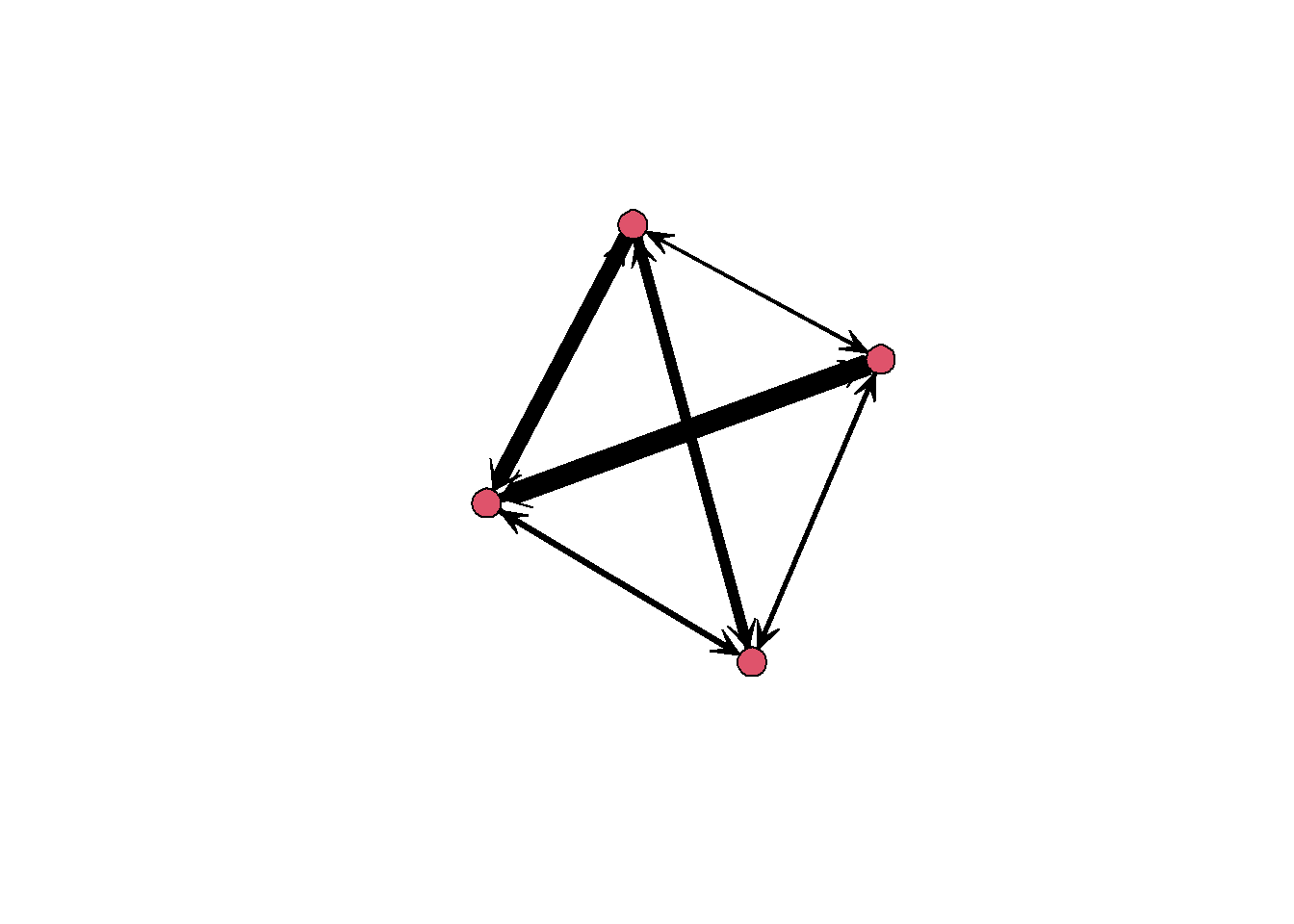
Unipartite vs. bipartite networks
Another commonly encountered type of network are bipartite (or bimodal) networks. In a bipartite network, there are two different kinds of nodes and only nodes of different kinds can be connected through an edge.
A classical example of this is a network of event attendances where the two different sets of nodes represent people and events, respectively, and edges indicate that a person attended an event.
Bipartite networks are easily represented with a regular edgelist:
edgelist <- data.frame(
  person = c("A", "A", "A", "B", "B"),
  event  = c("X", "Y", "Z", "X", "Y")
)
To construct a network object, we can pass this to the network constructor alongside the bipartite = TRUE flag:
net_bipartite <- network(edgelist, bipartite = TRUE, directed = FALSE)
net_bipartite
Network attributes:
vertices = 5
directed = FALSE
hyper = FALSE
loops = FALSE
multiple = FALSE
bipartite = 2
total edges= 5
missing edges= 0
non-missing edges= 5
Vertex attribute names:
vertex.names
No edge attributesThe bipartite = 2 in the printed summary indicates the number of nodes in the first partition.
Projecting bipartite networks
There are two unipartite networks we could create from our bipartite network by projection:
- A network of events which indicates whether two events were visited by the same people.
- A network of people which indicates whether two people attended the same events.
We can obtain both of these with a little bit of linear algebra on the incidence matrix, which, as opposed to a regular adjacency matrix, is not necessarily quadratic anymore:
inc <- as.matrix(net_bipartite)
inc
X Y Z
A 1 1 1
B 1 1 0If we multiply this matrix with its transpose, we obtain a weighted adjacency matrix representing the co-attendance count for the two people in the network:
inc %*% t(inc) A B
A 3 2
B 2 2If we change the order of the factors in the product, we obtain the co-attendance matrix for events:
t(inc) %*% inc X Y Z
X 2 2 1
Y 2 2 1
Z 1 1 1We can then proceed to create networks from these, as for regular weighted adjacency matrices.
Plotting bipartite networks
We can use the bipartite nature of this network for plotting by passing the gmode = "twomode" flag to the gplot(...) function. This will show the two sets of nodes in different colors and with different symbols:
gplot(net_bipartite, gmode = "twomode", usearrows = FALSE)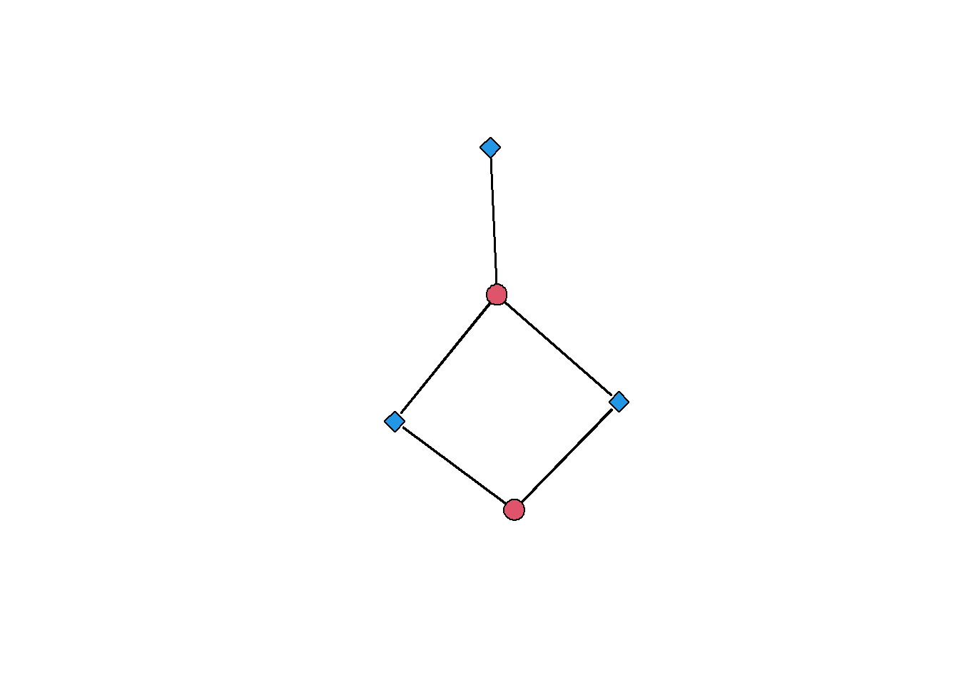
Exercises
Load the advice network in the file
data/lazega_advice.csvinto a directed network object.# Write your code here...Symmetrize the network using the weak rule.
# Write your code here...Symmetrize the network using the strong rule.
# Write your code here...Plot the symmetrized network next to the original with the correct arguments for an undirected network.
par(mfrow=c(1,2)) # DON'T CHANGE THIS

# Write your plotting functions here...
Compare the two symmetrized variants visually and in terms of their basic properties. What do you observe?
# Write your code here...