Representing networks in R

Networks can be represented in various formats, each offering its own advantages: Edgelists, for example, are good for storing and passing around networks, while adjacency lists or adjacency matrices are often preferable for computation.

Software packages for network analysis, such as statnet or igraph, usually hide the underlying data structure used for computation as an implementation detail while allowing import and export from/to a wide range of formats.

In the following, we will make use of the network and sna R packages to explore conversion from and to a range of network representations:

# uncomment the line below if you have not yet installed the packages
# install.packages(c("network", "sna"))

library(network)
library(sna)

The edgelist

The simplest way to represent a network is as a list of edges, aptly called an edgelist. We can store such an edgelist as a table with two columns where each row represents an edge and the first column holds the sender and the second column the receiver of an edge.

In R, one way to represent this would be a data.frame:

edgelist <- data.frame(sender = c(1,1,1), receiver = c(2,3,4))
edgelist

  sender receiver
1      1        2
2      1        3
3      1        4

Usually, we don’t use this edgelist for computing a measure of interest directly. Instead, we convert it to the network type defined in the network package (which is contained in the statnet suite):

net1 <- network(edgelist, directed = FALSE)

The network(...) function is quite smart and will often detect the appropriate format from the input argument. Data frames, e.g. will be treated as edgelists, while matrices will be treated as adjacency matrices. The function furthermore supports a wide range of arguments for specifying the kind of network that should be produced (e.g. directed vs. undirected).

If we print the produced network net1, it will show us some general information, such as the number of nodes and the number of edges, its basic properties and contained node and edge attributes:

net1

 Network attributes:
  vertices = 4 
  directed = FALSE 
  hyper = FALSE 
  loops = FALSE 
  multiple = FALSE 
  bipartite = FALSE 
  total edges= 3 
    missing edges= 0 
    non-missing edges= 3 

 Vertex attribute names: 
    vertex.names 

No edge attributes

We can pass this network object to the plethora of functions defined in the network and sna packages, such as gplot(...) to produce a plot of the network graph:

gplot(net1, gmode = "graph", label = 1:4)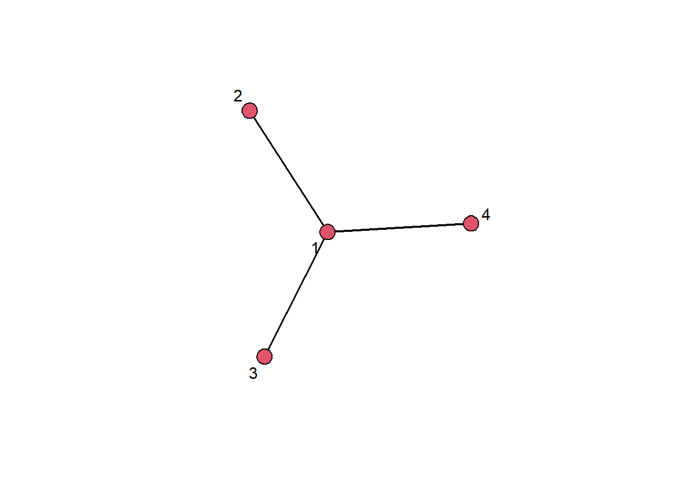

The adjacency matrix

A second important representation of a network is the adjacency matrix. For a network of size \(N\) (i.e., a network with \(N\) nodes), the adjacency matrix is a \(N \times N\) matrix (i.e., a matrix with \(N\) rows and columns). In this matrix, the cell indicated by the \(i\)th row and the \(j\)th column is \(1\) if there is an edge from node \(i\) to node \(j\) and \(0\) otherwise (for the case of an unweighted network).

In R we could construct an adjacency matrix manually using the matrix(...) function:

adjmat <- matrix(data = c(0,1,1,1, 
                          1,0,0,0, 
                          1,0,0,0, 
                          1,0,0,0), nrow = 4, ncol = 4, byrow = T)

adjmat

     [,1] [,2] [,3] [,4]
[1,]    0    1    1    1
[2,]    1    0    0    0
[3,]    1    0    0    0
[4,]    1    0    0    0

As before for the edgelist, we can pass this matrix to the network(...) function to construct a network object from the adjacency matrix:

net2 <- network(adjmat, directed = FALSE)

We can again print and plot this network object to see that it has the same structure as net1, which was constructed from an edgelist representing the same network:

net2

 Network attributes:
  vertices = 4 
  directed = FALSE 
  hyper = FALSE 
  loops = FALSE 
  multiple = FALSE 
  bipartite = FALSE 
  total edges= 3 
    missing edges= 0 
    non-missing edges= 3 

 Vertex attribute names: 
    vertex.names 

No edge attributes

 gplot(net1, gmode = "graph", label = 1:4)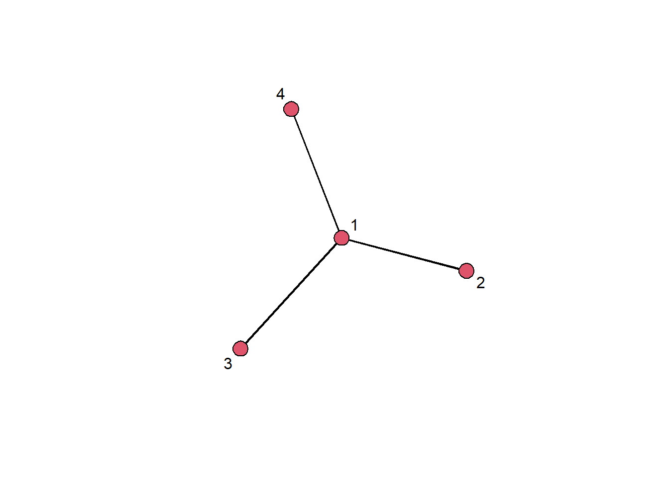

Indexing into an adjacency matrix

A couple of sessions ago, we saw how to index into a vector using square brackets (e.g. myvec[1]). We can do the same for our adjacency matrix, using two indices (the first for the row and the second for the column):

adjmat[1,2]

[1] 1

This tells us that there is an edge in our network from node 1 to node 2.

Indexing into the network is even directly supported for network objects, using the same indexing syntax:

net1[1,2]

[1] 1

Reading an adjacency matrix from a csv file

We can also read an adjacency matrix that is stored in a .csv file using, e.g., the built-in read.table(...) function. Here, we need to pass some additional arguments because the file contains row names in the first column (thus we specify row.names = 1) and uses numeric names, which by default are invalid (so we pass check.names = FALSE).

adjmat <- read.table("data/lazega_advice.csv", 
                     sep =";", 
                     header = TRUE, 
                     row.names = 1, 
                     check.names = FALSE)

Because adjmat is a data frame right now but we usually want to represent an adjacency matrix with R’s built-in matrix type, we need to convert it first:

adjmat <- as.matrix(adjmat)

We can check that the matrix is quadratic (i.e. has as many rows as it has columns):

nrow(adjmat) == ncol(adjmat)

[1] TRUE

and that the column names are equal to the row names:

all(colnames(adjmat) == rownames(adjmat))

[1] TRUE

Now that we have done some validation that we loaded the data correctly, we can pass the adjacency matrix to the network(...) function to construct a network:

net <- network(adjmat, directed = TRUE)

There and back again

R and the network package allow us to also go the other way, e.g. creating an edgelist from a network object. We can do this by converting the network to a data frame using as.data.frame(...):

el <- as.data.frame(net1)
el

  .tail .head
1     1     2
2     1     3
3     1     4

Here, the .tail column holds the sender for each edge and .head the receiver.

We can similarly also convert to an adjacency matrix:

adj <- as.matrix(net1)
adj

Exercises

Load the adjacency matrix contained in the file data/lazega_advice.csv into R.
```
# Write your code here...
```
Create an undirected network from the adjacency matrix.
```
# Write your code here...
```
How many nodes and edges does the network have?
```
# Write your code here...
```
Plot the network. Color the nodes black and the edges grey.
```
# Write your code here...
```
Get the edgelist for the network and write it to a .csv file.
```
# Write your code here...
```
Index into the adjacency matrix to find out whether node 2 and node 4 are connected.
```
# Write your code here...
```