Krackhardt’s EI-index

A simple way to quantify group structure is the EI-index proposed by Krackhardt & Stern (1988). It measures the degree to which a network tends to be concentrated on within- or between-group relationships and is defined as the difference of External (i.e., edges between groups) and Internal (i.e., edges within groups) edges divided by the total edge count: \[ \frac{E-I}{E+I} \]

The EI-index can be computed for the full network, for each group separately, or even for individuals. In the latter case, the EI-index indicates the tendency of a person to establish ties to persons in other groups rathern than to other members of their own group. Its bounds are typically -1 (all edges internal) and 1 (all edges external), although there can be degenerate cases when group sizes differ strongly.

In the following we again use office affiliations of Lazega’s lawyers to demonstrate the EI-index.

Loading data

As usual, we start by loading packages and data:

library(statnet)

adjmat <- read.table("data/lazega_advice.csv", 
                     sep =";", 
                     header = TRUE, 
                     row.names = 1, 
                     check.names = FALSE)

adjmat <- symmetrize(as.matrix(adjmat))
net <- network(adjmat, directed=FALSE)

Note that we symmetrize the network because the EI-index is by default only defined for undirected networks. We also need to load the attribute data again:

attrib <- read.csv2("data/lazega_attrib.csv")

Computing the EI Index

The EI-index is not implemented in statnet but easy enough to implement so that we can roll our own. The file helpers/EI_index.R contains the function EI_index(...) which computes the index at all three levels. We can make it available via source(...):

source("helpers/EI_index.R")

Calling the function EI_index(...) on a network object and a grouping vector returns a list of results:

res <- EI_index(net, attrib$office)

We can access the EI-index results for the different levels via $:

res$global

[1] -0.5481172

This tells us that there is a quite strong tendency towards intra-office connectivity.

For group-level and individual-level results, we get a dataframe which also contains membership counts and the raw counts of external and internal ties:

res$group

  group  N   E   I         EI
1     1 48 153 896 -0.7082936
2     2 19 137 206 -0.2011662
3     3  4  34   8  0.6190476

As we can see, offices 2 and 3 are much more ‘extroverted’ than group 1.

Permutation Test for Global EI Index

To assess whether the observed EI index is larger than could be expected under some null model, we can compare it to the values we get for networks simulated from said null model. This involves creating a large number of networks with similar basic features (size, number of edges, degree distribution) and computing the EI-index for each one of these, thus creating a reference distribution:

# Create 500 random permutations of our network
pg <- list()
for (i in 1:500) pg[[i]] <- network(rmperm(net), directed=FALSE)

# Calculate EI index for each permuted network
ei_perm <- sapply(pg, EI_index, attrib$office, out="global")

# Plot the distribution of permuted EI indices
hist(ei_perm, xlim=c(-1, 1), xlab="EI-Index", main="Permutation test for EI-Index")
abline(v = res$global, col = "red", lwd = 2, lty = 2)
legend("topright", legend="observed", col="red", lty=2)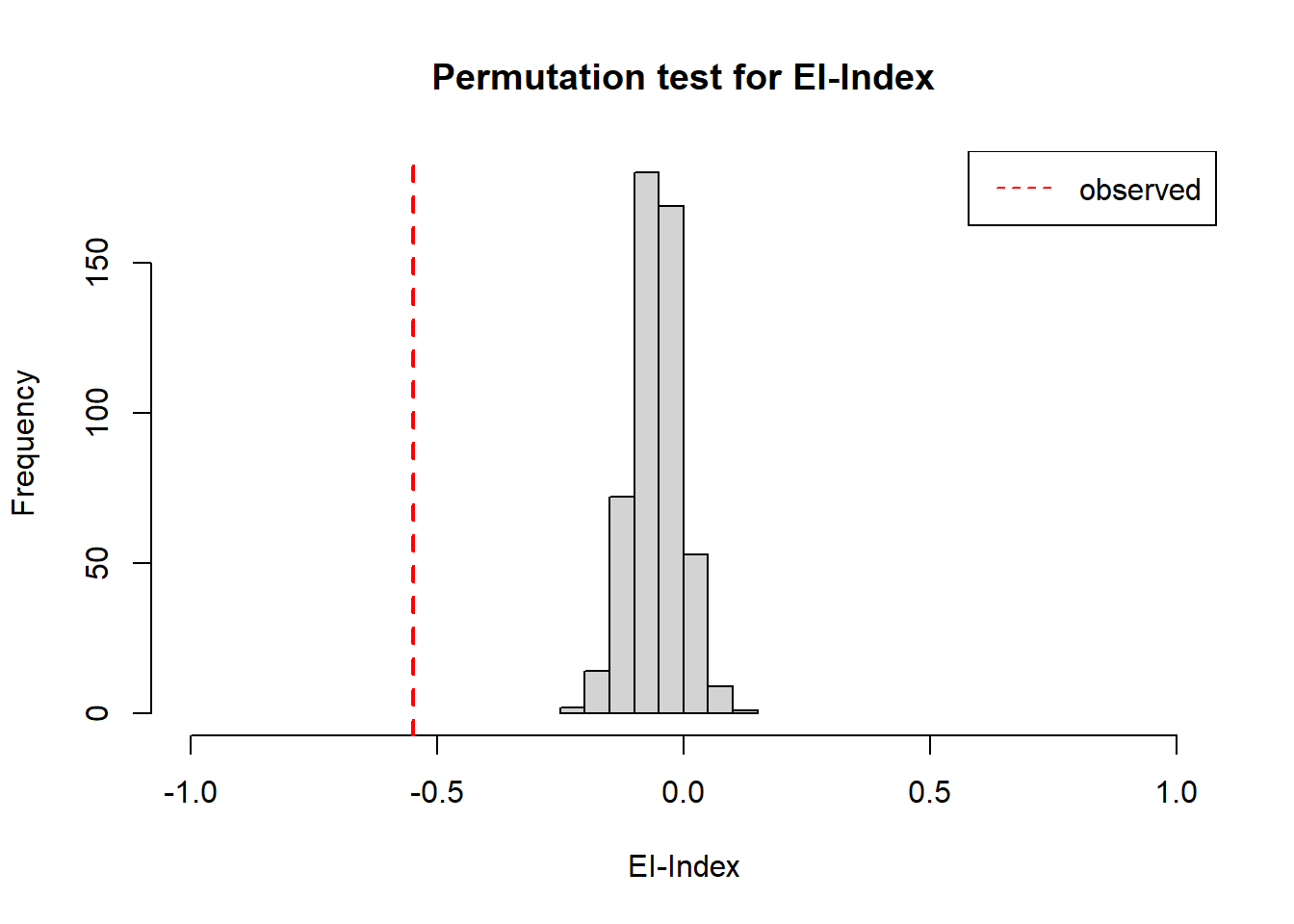

As we can see, the observed EI-index decidedly smaller than in the randomly generated networks and so we can conclude that our grouping variable (office affiliation) does play some role for shaping network structure.